Introduction
Computational Fluid Dynamics (CFD) programs are powerful tools that allow engineers to simulate and analyze fluid behavior in a wide range of scenarios. From water flow to high-speed gases, these programs let you study dynamic systems in detail, which saves you time and money before you build physical prototypes.
Some common applications include:
- Analyzing the aerodynamics of F1 cars, airfoils, or wind turbines.
- Simulating heating, air conditioning, and ventilation systems.
- Studying heat transfer and thermal management.
- Modeling turbomachinery such as turbojets or rocket nozzles.
Recently, I used one of these programs to compare and analyze two distinct rocket nozzle geometries to determine which is more efficient and optimal. In this article, I’ll guide you through the entire process: modeling, meshing, simulating, and interpreting the results of a CFD simulation.
About Rocket Nozzles and their shape
Before diving into the software, it’s important to understand the unique geometry of a rocket nozzle. Unlike aircraft engines, rocket gases reach supersonic speeds to provide the necessary thrust for exiting the atmosphere. At these velocities, gas behavior changes dramatically; it can be explained by the continuity equation and the Area-Mach number relation, a simplified differential form is:
$$ \frac{\mathrm{d} A}{A} = (M^2 - 1)\frac{\mathrm{d} V}{V} $$
- At subsonic speeds (M < 1): fluids are accelerated by decreasing the area.
- At supersonic speeds (M > 1): fluids are accelerated by increasing the area.
This is why we need a convergent-divergent nozzle, also known as Laval Nozzle.

As shown in the image, gases move at subsonic speeds in the convergent section of the nozzle. Only upon reaching the throat do they accelerate to supersonic speeds, requiring a divergent geometry. The behavior of supersonic fluids is a fascinating topic: learn more about it and its shock waves here.
Unlike rocket engines, jet engines typically use only a convergent nozzle because their exhaust gases remain subsonic.
About Ansys Fluent and CFD software
ANSYS Inc is a multinational company that develops engineering simulation software for industries ranging from automotive to construction. It’s one of the leaders in its field. For this project, I used Ansys Fluent, their solution for CFD applications. I chose ANSYS because:
- It’s highly regarded by universities and researchers.
- It handles turbulent flow models exceptionally well.
- It offers a free student license.
When working with CFD software, the typical workflow is:
- Designing the 3D or 2D model, using Ansys Designer or any CAD software.
- Meshing: generating a mesh for your model; the program will perform the calculations on each segment.
- Computing: the software evaluates its mathematical models.
- Analyzing and interpreting the results to draw conclusions.
Creating the model
We begin by creating the nozzle itself. For reference, I used the dimensions of the famous J-2S engine, used in several Apollo missions. The geometry has been generated in Ansys Design Modeler, including a free space to simulate the behavior of gas and air.
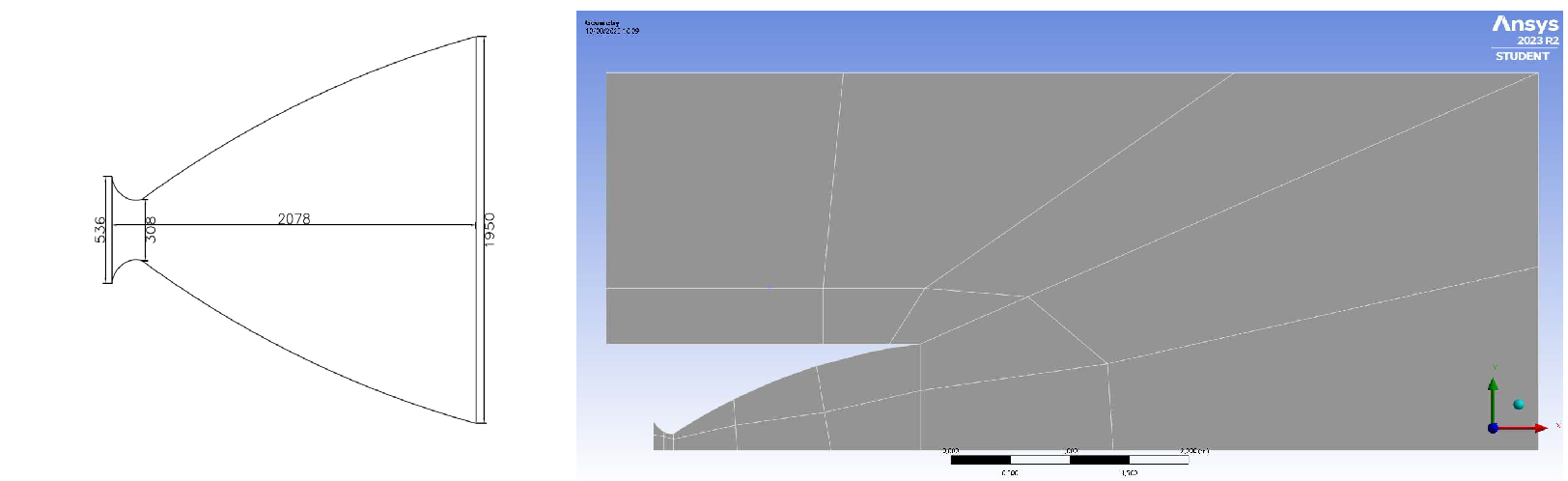
Note that only half of the nozzle is designed, as a symmetry plane can be specified later. The geometry is divided into smaller segments to prepare for meshing, with finer divisions in areas requiring higher accuracy, mainly inside the nozzle.
Meshing the nozzle
The next step is to generate a mesh using Ansys Meshing. In this case, I used quadrilaterals due to the regular geometry and a fixed subdivisions method. By selecting all edges and applying edge sizing (left image) with 50 divisions, each edge is split into 50 parts. Then, a face meshing is applied, setting the method to quadrilaterals. Clicking generate automatically divides each face into smaller faces based on the edge divisions.
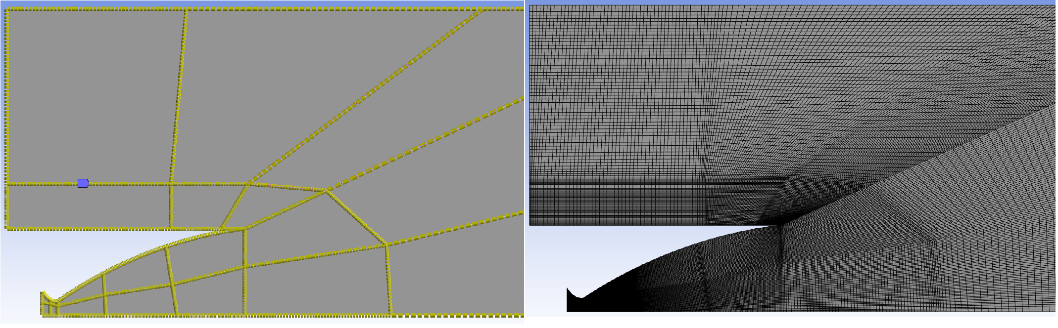
The result, shown on the right, is a mesh with over 50,000 segments.
Running Ansys Fluent
The next step is to set up the simulation in Ansys Fluent. The software offers a wide range of settings, but I’ll focus on the most important ones. First, we define the properties of the fluid to be analyzed: the product of combusting liquid oxygen with hydrogen. According to NASA’s data, under Materials > Fluid, we set up a compressible ideal gas with:
- Density [kg/m³]: ideal-gas
- Cp (Specific Heat) [J/(kg·K)]: 3992 (constant)
- Thermal Conductivity [W/(m·K)]: 0.0242 (constant)
- Viscosity [kg/(m·s)]: 1.34e-05 (constant)
- Molecular Weight [kg/kmol]: 12 (constant)
For the solid material, a simple aluminum model is used:
- Density [kg/m³]: 2719
- Cp (Specific Heat) [J/(kg·K)]: 871 (constant)
- Thermal Conductivity [W/(m·K)]: 202.4 (constant)
Next, we define the boundary conditions by selecting the edges corresponding to each condition:
- Inlet (blue arrows): where the gas enters the nozzle.
- Symmetry: the horizontal edge serving as the symmetry line.
- Wall: the nozzle wall, assigned the aluminum material.
- Outlet (red arrows): where the gas exits the simulation.
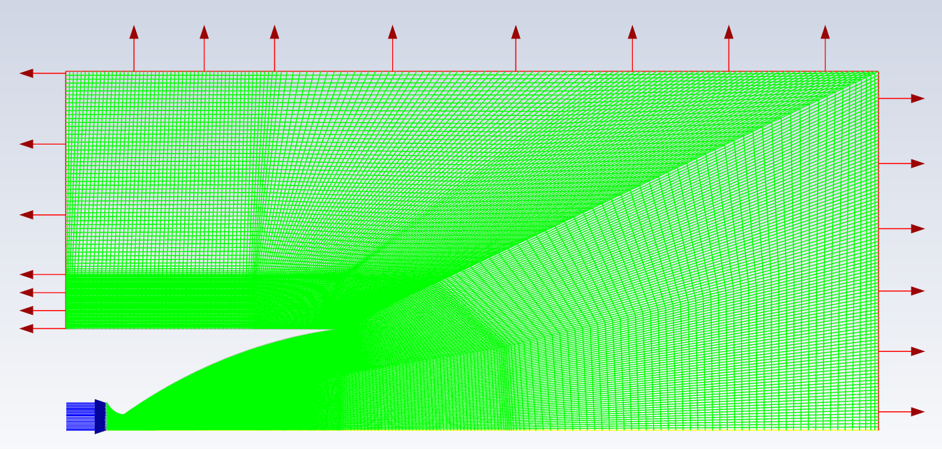
For this simulation, I modeled an atmospheric flight, setting the outlet pressure and temperature to 11,000 Pa and 200 K (corresponding to 10.8 km above sea level), and the inlet pressure and temperature to 530,000 Pa and 3,500 K (full engine thrust).
You can modify these values to simulate other scenarios, such as ignition, or conditions near the Kármán line (~100 km altitude).
Simulating gas speeds
A key step is specifying what you want to observe. In this case, I created a contour under Results > Graphics > Contours to visualize the Mach number of the gas particles. Other options like pathlines or particle tracks are available, but contours are best for visualizing velocities.
For high-speed gases, focus on Mach number rather than absolute speed. Mach number depends on temperature and other factors, and it determines whether the flow behaves in a subsonic or supersonic way.
Now, the simulation is ready to run. Start with 80 iterations and adjust as needed based on the relative error per iteration. Even after running a simulation, you can add more iterations to refine the results. Here’s an example of the error after several iterations and the resulting Mach number distribution:
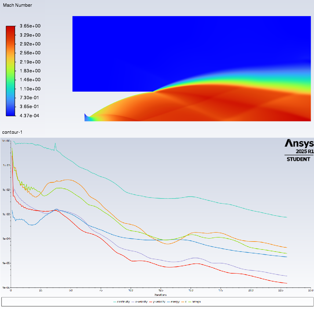
With around 100 iterations, the error is acceptable (residuals around 1e-04 or 1e-03) and the results are accurate. As an extra step, you can post-process the results in Fluent or Fluent Post: add symmetry, adjust the colormap, set minimum and maximum values, etc. Check out this guide for more information.
Further simulation
To showcase the power of these tools, I compared the NASA-designed nozzle with a custom nozzle featuring an outlet three times smaller. Simulations were run at different altitudes (up to 15 km) to model the early stages of a rocket flight.
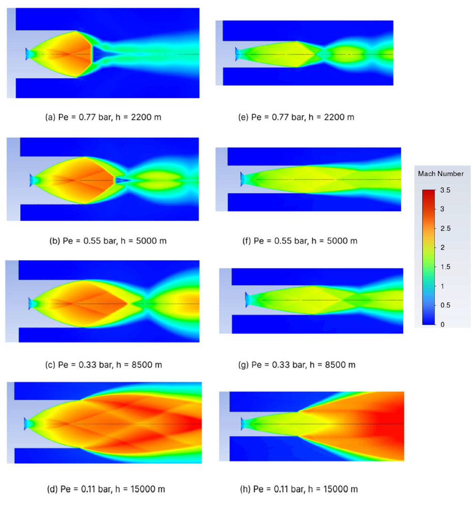
At low altitudes, both nozzles exhibit overexpanded flow (the nozzle is too large for the ambient pressure). Distinct shock structures appear, such as normal shock waves (images a and b) and oblique shock waves (mainly in image c). At higher altitudes, the opposite effect occurs: underexpanded flow (the nozzle is too small), especially in the second nozzle.
Shock diamonds are visible in the first nozzle and, to a lesser extent, in the second. These shock wave patterns are also seen in jet engines - check out this video for a real-life example.
While shock waves are visually striking, intense shock interactions lead to energy losses. Thus, although the first nozzle delivers a greater absolute thrust and is ideal for rocket launches, the second nozzle is more energy efficient (because the energy losses due to shok waves are minimum) but it also produces less thrust overall and would be better suited for a space shuttle, for example.
Although the results provide a valuable first impression, more advanced simulations (including variable thermodynamic properties and 3D turbulence models) would be required for higher fidelity.
Conclusions
As we have seen, CFD simulations with ANSYS Fluent provide interesting tools to improve rocket nozzle design, allowing engineers to optimize geometry for specific flight conditions. The fact that we can visualize complex phenomena like overexpanded and underexpanded flows, shock waves, and energy losses shows that CFD software is a really useful tool that provides results accurate with reality, which highlights its importance.
To sum up, these tools not only accelerate the design process but also contribute to making the process of innovating and experimenting with propulsion systems safer and more efficient. If you are more interested in the topic or have any doubt, don’t hesitate to reach me out: mageche10@gmail.com
References
- THEORETICAL & CFD ANALYSIS OF DE LAVAL NOZZLE by D. DESHPANDE, S. VIDWANS and others.
- Historia de la dinámica de fluidos computacionales. by A. González.
- CFD ANALYSIS OF CONVERGENT-DIVERGENT NOZZLE by G. SATYANARAYANA, Ch. VARUN and S.S. NAIDU