Introduction
Did you know that most artificial satellites orbit around empty points in space? These points are called Lagrange points, and they allow for enormous fuel savings. They are also reference locations for space telescopes such as the James Webb and GAIA. In recent years, these points have attracted a lot of attention in the aerospace industry.
My colleagues and I have decided to study a specific type of orbit (Lyapunov orbits) for a specific case of the three-body problem. In this post, I’ll explain the mathematics behind this study and how we solved it using MATLAB.
Theoretical Background
Before starting, it’s important to understand some key concepts.
Circular Restricted Three-Body Problem
The Circular Restricted Three-Body Problem (CR3BP) is a special case of the Three-Body problem where two primary masses are much larger than the third, which is considered negligible. We also assume that the two main bodies orbit in circles around their common center of mass. To describe the system, we use the parameter
$$\mu = \frac{m_2}{m_1 + m_2} $$
In our study, we focus on the symmetric case, where both primary objects have equal mass: \( m_1 = m_2 \implies \mu = 0.5 \). This means the center of mass is exactly halfway between the two large bodies.
Lagrange Points
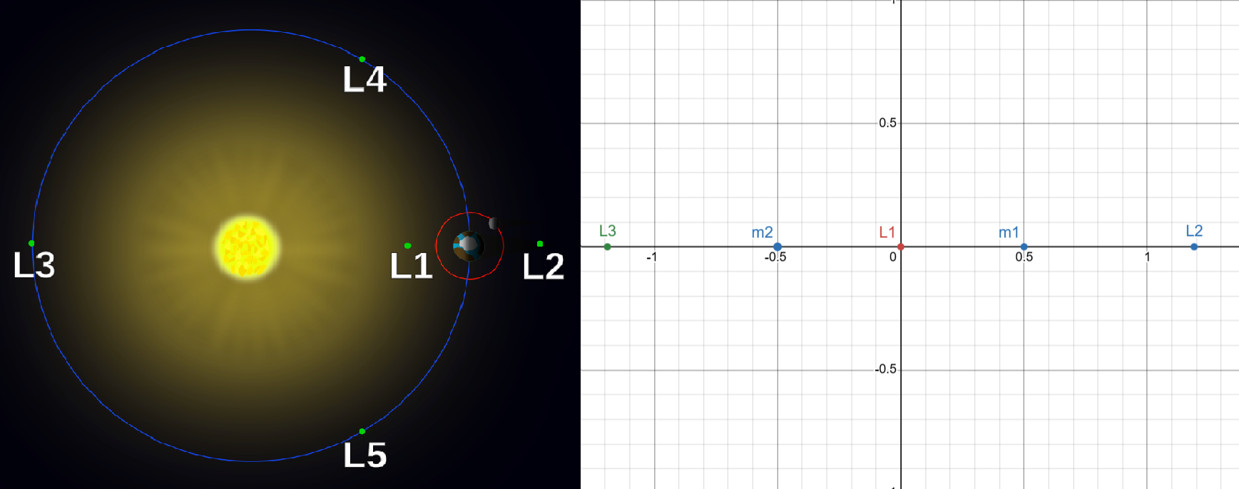
Due to the gravitational pull of the massive bodies and the system’s rotation, there are five points where gravity and the Coriolis force balance each other. Three of them are the unstable Lagrange Points (L1, L2, and L3). In theory, an object could remain at these points indefinitely without expending energy. However, even the slightest disturbance can make it drift away unpredictably. There are also two stable Lagrange Points, L4 and L5, but we won’t cover those here.
In our symmetric case, the two large masses are at \( (0.5, 0) \) and \( (0, 0.5) \). The unstable Lagrange Points can be found by solving:
$$x - \frac{(1-\mu)(x+\mu)}{(|x+\mu|)^3} - \frac{\mu (x- (1-\mu))}{|x - (1-\mu)|^3} = 0 $$
I’ll explain this equation later. The following image shows a general diagram of the Lagrange Points and highlights the three unstable points we are studying.
Halo and Lissajous Orbits
Satellites and space telescopes often take advantage of the unstable Lagrange Points L1 and L2. Since no object can remain at these unstable spots on its own, we guide them into special paths called Halo or Lissajous orbits. These orbits allow spacecraft to stay near these regions with minimal fuel consumption. What’s fascinating is that a satellite seems to circle around “nothing”—a point in empty space. When dealing with unstable points like L1, L2, or L3, engineers must carefully choose initial conditions to minimize the energy needed for long-term corrections.
Our goal is to find these initial conditions for the symmetric system, specifically for Lyapunov orbits, which are 2D elliptical orbits around L1.
Analytical Problem
As mentioned, the two main forces in the system are gravity and the force due to rotation. The acceleration of the third object due to gravity is:
$$ \boldsymbol{a_g} = - \frac{G m_1}{(\boldsymbol{r} - \boldsymbol{r_1})^2} - \frac{G m_2}{(\boldsymbol{r} - \boldsymbol{r_2})^2} $$
When we also include the centrifugal and Coriolis forces, the acceleration vector becomes:
$$ \boldsymbol{\ddot{r}} = \boldsymbol{a_g} + 2 \boldsymbol{\omega} \times \boldsymbol{\dot{r}} + \boldsymbol{\omega} \times (\boldsymbol{\omega} \times \boldsymbol{r}) $$
We can define the effective potential \( \Omega \) as:
$$ \boldsymbol{\ddot{r}} = \nabla \Omega - 2 \boldsymbol{\omega} \times \boldsymbol{\dot{r}} $$
So, with \(r = (x^2+y^2)\); \(r_1 = |x+\mu|\) and \(r_2 = |x-(1-\mu)|\), we get:
$$ \Omega = \frac{1}{2} \omega^2 r^2 + \frac{G m_1}{r_1} + \frac{G m_2}{r_2} $$
Finding the Lagrange Points and Their Stability
We know that the three unstable Lagrange points are aligned along the axis \(y = 0\). Therefore, we can find these points by solving:
$$ \frac{\partial \Omega}{\partial x} = \ddot{x} - 2 \dot{y} = 0 $$
This leads to the equation mentioned earlier in the Lagrange Points section.
To determine whether these points are unstable, we use the linearization method (linear stability analysis).
In nonlinear dynamical systems, one of the standard ways to study the stability of an equilibrium point is through linear stability analysis. The idea is simple: you first find the equilibrium, then compute the Jacobian matrix of the system at that point, and finally look at its eigenvalues.
If any eigenvalue has a positive real part, it is unstable.
The Jacobian matrix for our system is:

By substituting the second derivatives for each Lagrange point and using MATLAB’s eig command to find the eigenvalues, we see that each point has at least one eigenvalue with a positive real part—confirming their instability.
Searching for Periodic Solutions
Our main objective is to find 2D periodic orbits around L1. In other words, we want solutions of the form:
$$x(t) = \alpha \cos(\omega t); \quad y(t) = \alpha k \sin(\omega t)$$
We start by finding solutions for the linear approximation of the nonlinear system. For a given amplitude \(\alpha = x_0\), we look for an initial vertical speed such that the solution to this IVP (Initial Value Problem) crosses the symmetry axis \(y = 0\) perpendicularly. So, our object starts at:
$$ (x, y, \dot{x}, \dot{y}) = (\alpha, 0, 0, \alpha k \omega) $$
If we get the eigenvectors corresponding to the complex eigenvalues (periodic behavior) of the Jacobian matrix at L1, we obtain:
$$ v_\pm = (- 0.0728, \pm 0.3195 i , \pm 0.2099 i , 0.9212)$$
Dividing the values corresponfig to \(x\) and \(\dot{y}\), we find first relation between \(x_0\) and \(\dot{y}_0\):
$$ \frac{\alpha k \omega}{\alpha} = \frac{0.9212}{-0.0728} = - 12.654 \Rightarrow k \omega \approx - 12.654 $$
We use the eigenvectors corresponding to the complex eigenvalues because, usually, in linear systems, these are the vectors used to find periodic or quasi-periodic solutions. Although we can’t be one hundred percent sure that it is correct to pick these vectors, we will see in the numerical part that our linear approximation is quite good.
Numerical Solution
Now, our problem is to find those initial states for each \(x_0 = \alpha\) that produce periodic orbits numerically.
We’ll use MATLAB’s ode45 and ode78 methods, which are based on Runge-Kutta algorithms.
MATLAB Implementation
When implementing a nonlinear dynamical system (a system of differential equations) in MATLAB, the first step is to write the function that the solver will iterate—in other words, a function that, given the current state, returns the next state.
1 | function dXdt = sistemaEDOSs(t, X, mu) |
Next, we use MATLAB’s built-in event detection when solving systems with ode methods. In our case, we want to detect when the object crosses the horizontal axis—that is, when the second component of the system is zero. After that, we look for initial conditions that make the fourth component zero when the event triggers: the object will cross the axis perpendicularly.
1 | function dx1 = dxEny0(mu, x0, dy0) |
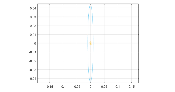
Once we’ve found a suitable initial vertical speed for a given position, we can run a full simulation and obtain an elliptical orbit around the L1 point (yellow star):
If we let the simulation run for a longer period of time, we see that, after two or three ellipses, the particle starts a chaotic movement.
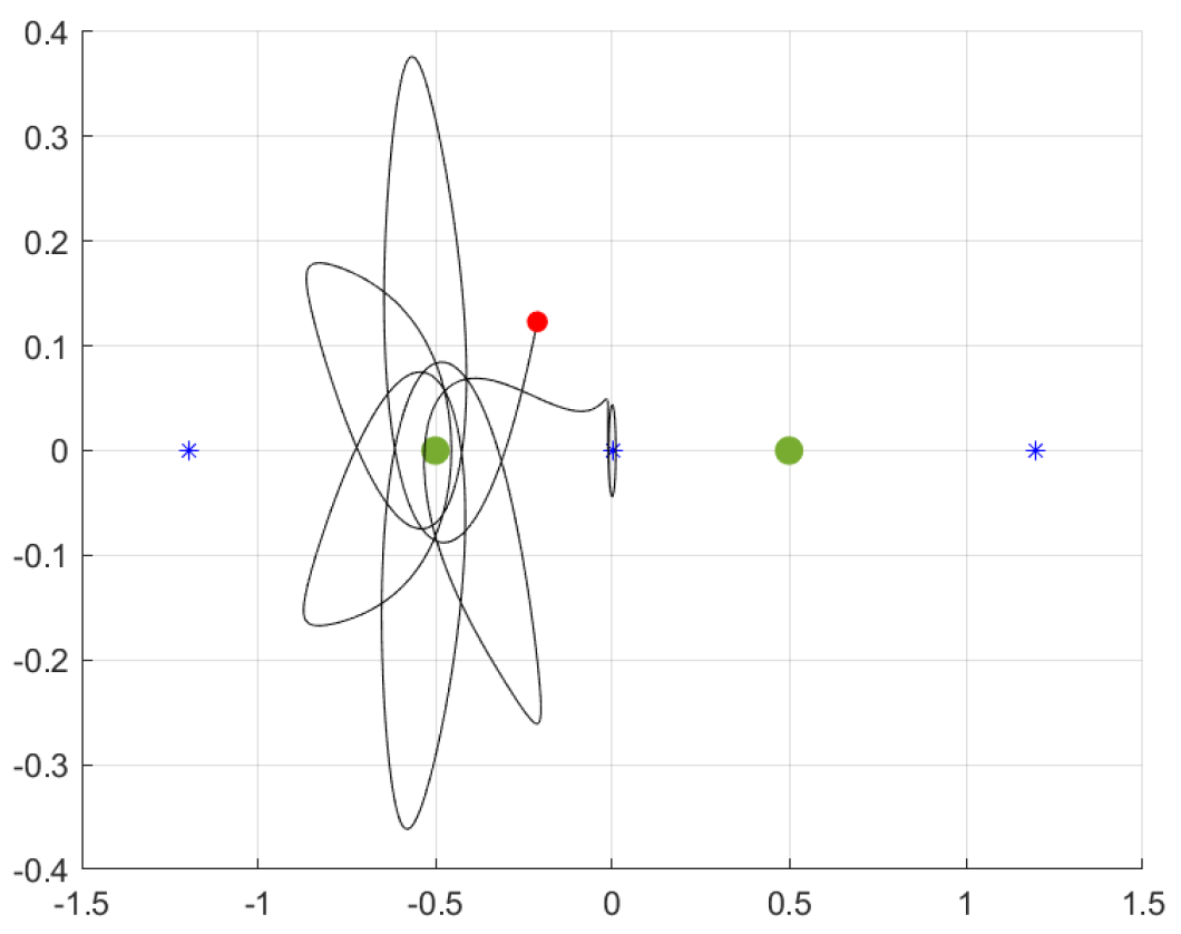
MATLAB only works with a maximum of 16 decimals of accuracy. Even with this little error, the particle starts moving unpredictably. This phenomenon illustrates the chaotic nature of the dynamic system and its instability. In the real world, the satellites using these orbits must be corrected by importing energy to the system (little engines, for example).
Correlation Between Amplitude and Initial Velocity
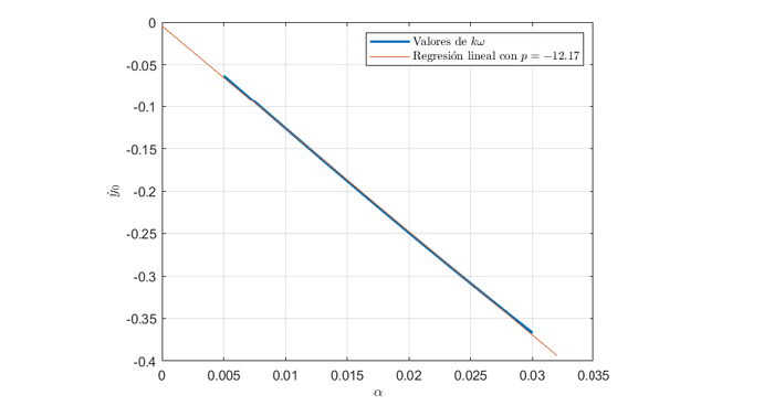
The next step is to run a series of simulations with amplitudes from 0.001 to 0.03 and, for each amplitude, find the initial vertical velocity that produces periodic orbits. As we’ve seen, this relation is:
$$ \dot{y}_0 = \alpha k \omega $$
By performing a linear regression on the numerical values, we can estimate \(k\omega\). In this case, it’s about -12.17, which is close to the value from the linear approximation.
Conclusions
After working on this project, we have acquired a deeper understanding of how satellites and space telescopes can maintain stable paths in regions of space that seem completely empty. We have also learned a lot about Lagrange Points and how the combination of theoretical analysis with numerical simulations in MATLAB can help to identify the initial conditions required for specific problems.
This approach demonstrates the practical value of mathematical modeling and computational tools in solving real-world aerospace problems. For this reason, big companies are spending lots of money on developing new and better tools. Moreover, now IA can be integrated into these tools to make the process faster and more reliable. If you’re interested in orbital dynamics, mission planning, or interested by the mathematics behind space exploration, Lyapunov orbits are a good starting point to dive into this world.
Much to my regret, I can’t go into the technical issues and mathematical rigor as much depth as I’d like in this post, so as not to make the article too long. If you’re interested in this topic and would like more information, please don’t hesitate to contact me: mageche10@gmail.com
References
- Points de Lagrange et Orbites de Halo by J. L. Coron
- The Lagrange Points by N. J. Cornishç
- Mecánica Orbital y Vehículos Espaciales by R. Vázquez
- Lagrange Image under CC License